I roughly learnt CNN recently and was about to code one just like the FCNN I coded before. However this may be too costly to time, so I'll use TensorFlow in this case and learn more about TF conveniently.

Convolutional Neural Network

(This is my first English blog, and maybe there would be more blogs in EN in the future if I'd like to practice my writing in English. My English sucks, so feel free to raise issues if any error is found)

CNN Introduction

Actually the core feature of convolutional neural network is the convolutional layer and maybe pooling layer. But actually pooling layer is usually treated as a part of convolutional layer since it does linear calculations.

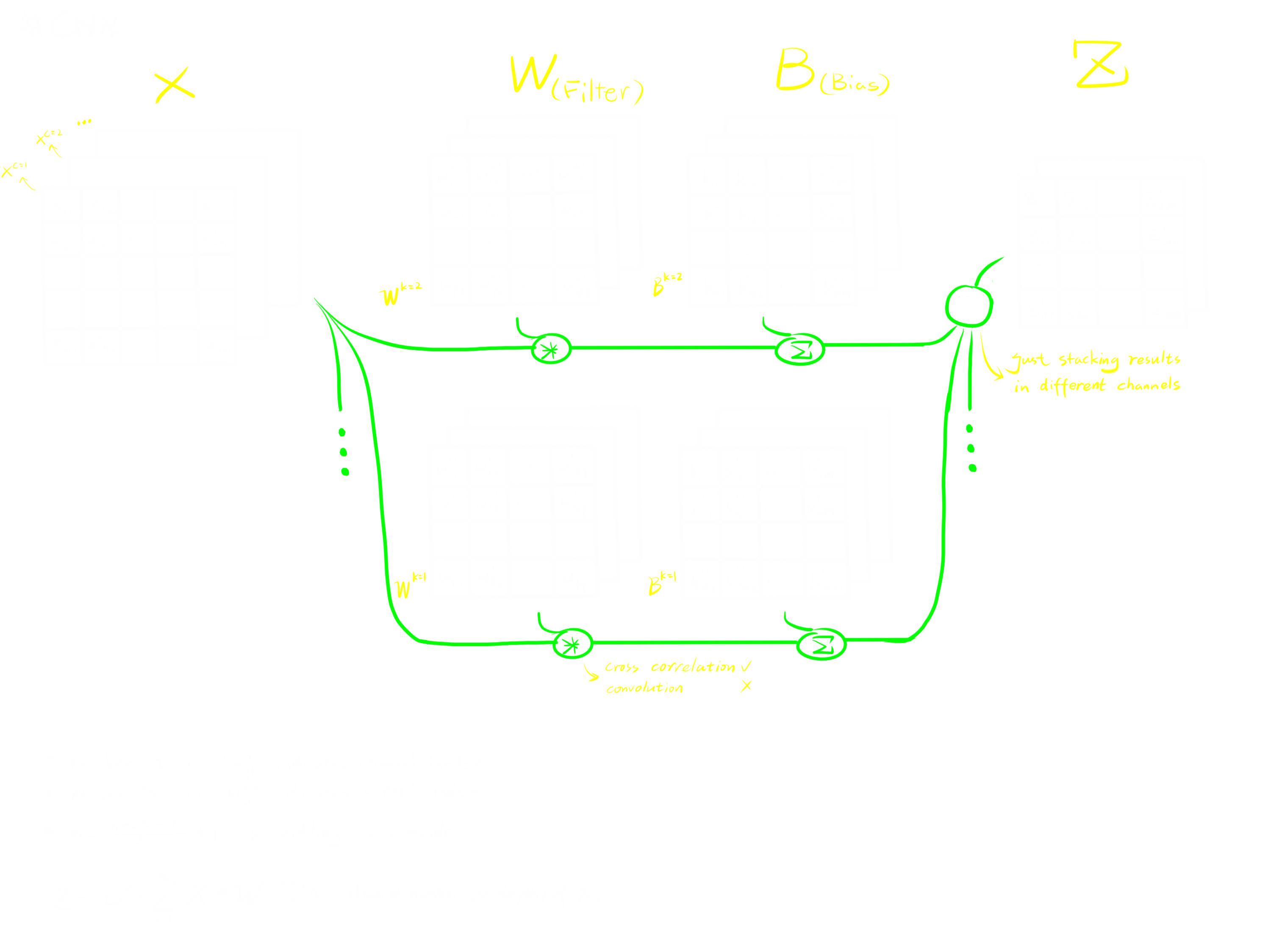
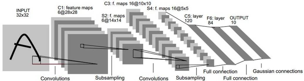
A convolutional layer can be concluded as following image, which was drawn by myself.

Structure

A convolutional layer has two parameter matrices we need to train, which are Filter and Bias. Being different from FC layer, in a convolutional layer, Bias matrix cannot be blended into Filter matrix due to the cross correlation operation.

Comparing with FC layers, the biggest change in convolutional layers is that convolutional layers take tensors as inputs, keeping the form of tensor from the beginning to the end. On the contrary, in the FCNN, we would usually reshape the input to a vector at first.

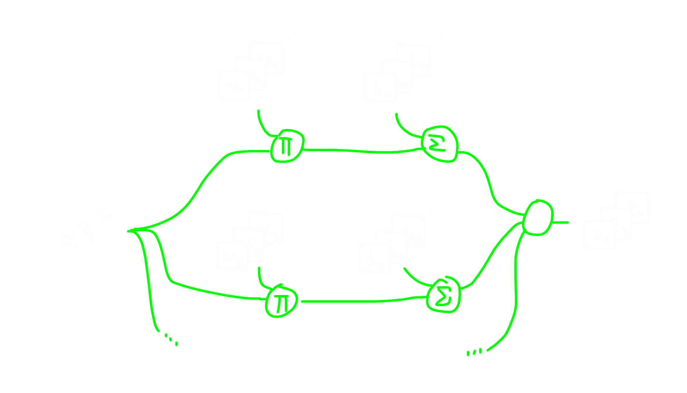
Mathematically, we can treat a FC layer as a special case of convolutional layer, and the convolutional layer is the generalization of the FC layer. To prove this, just making all matrices in convolutional layer one dimension. The following image can explain the conclusion further.

Working Flow

A convolutional layer feeds its input to convolutional kernels. The kernels will do cross correlation operation and add the bias accordingly. At the end, collect all outputs from all kernels and make it a new tensor by just stacking those outputs. The output of a convolutional layer is called feature map.

Goal

A convolutional layer has a rather different goal from the FC layer.

When using FC layers, we are expecting a humanoid brain neuron like model can learn from generic inputs. However, when doing image processing, this particular topic leads to huge amount of trainable parameters in FCNN. In which case, we can do some pre-process to the input image since we can easily see that not every pixel in the input is important for the task, and this pre-process is called convolution. From this aspect, we can treat convolutional layers in the network as feature detectors, the convolutional layers learn to extract meaningful features from the image using the filter and bias tensor, and use pooling layers to compress / emphasis the feature it extracted, making fewer trainable parameters.

But as I mentioned, convolutional layers are only good at feature extraction. So when doing classification with multiple features, it's still better to use FC layers. In which case, a CNN usually end up with FC layers to give the final outputs.

In conclusion, in CNN, the goal of a convolutional layer is extracting features from a rather huge input. The goal of a pooling layer is compressing data without damaging the main features. The goal of a FC layer in the end of CNN is to learn classification by giving features just as normal AI things would do.

Application

We can apply CNN in not only image recognition but also other area that shares the basic features with image recognition. For example, go and mahjong playing used CNN a lot. Especially in go playing, we can treat the go board as a 19x19 image with 48 channels (the reason why there should be 48 channels was raised by pros). and we can process every local part separately to get features of current situation. However, pooling layers are NOT used in go AI since the data loss in pooling operation is deadly to describe a go game. So design your CNN structure thoughtfully before putting it into training.

Back Prop

I used to be quite curios about the back propagation in convolutional layer, and pooling layers also made me confused. But actually they are basically the same as back prop in FCNN if you expand all formulas.

This Video explained how back prop in convolutional layer works.

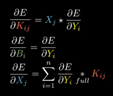
As for max pooling, since it's just doing linear calculation, when doing back prop, just implement the gradient to the max A of the previous one if there is a max pooling layer between them, and others' gradients are 0.

CNN Example

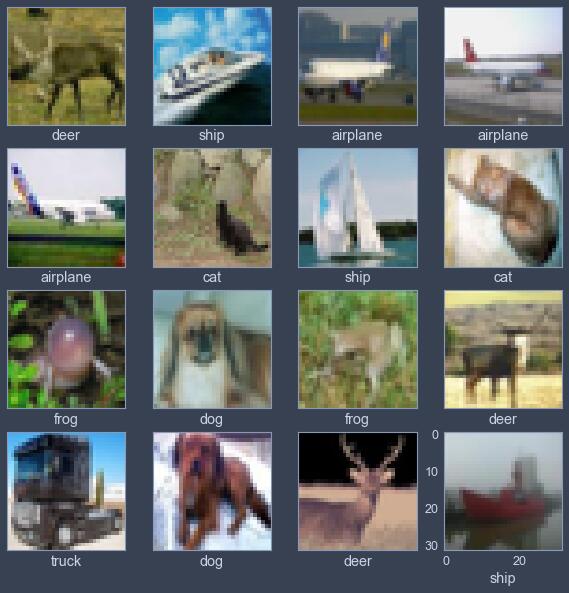
Following this video, I coded a simple CNN example with TensorFlow to classify CIFAR10, a dataset with 10 classes as following.

'airplane', 'automobile', 'bird', 'cat', 'deer', 'dog', 'frog', 'horse', 'ship', 'truck'

However, in my opinion, some images are too blur to classify even for human, so it's not surprised that AI performs poorly.

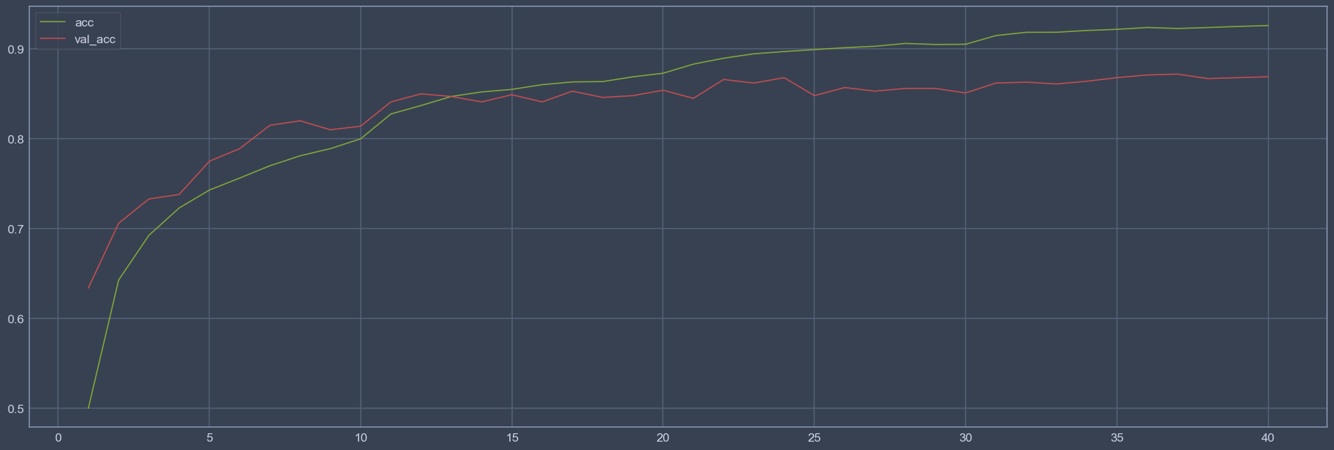
Though there's somebody made accuracy 90%+ AI with ResNet, that should be the content of another blog then. I made it 86.0% in 40 epochs, which is enough for experimenting CNN.

Structure

Referring LeNet, VGG, and so on, we can see that the width and length of the tensor tend to go down, whereas the number of channels does increase as we go deeper into the layers of the network. Another pattern that still often repeated today is that we might have some one or more conv layers followed by a pooling layer.

So I came up with this structure:

1
2
3
4
5
6
7
8
9
10
11
12
13
14
15
16
17
18
19
20
21
22
23
24
25
26
27
28
29
30
31

Model: "sequential"
_________________________________________________________________
 Layer (type)                Output Shape              Param #   
=================================================================
 conv2d (Conv2D)             (None, 32, 32, 64)        1792      
                                                                 
 max_pooling2d (MaxPooling2D  (None, 16, 16, 64)       0         
 )                                                               
                                                                 
 conv2d_1 (Conv2D)           (None, 16, 16, 128)       73856     
                                                                 
 max_pooling2d_1 (MaxPooling  (None, 8, 8, 128)        0         
 2D)                                                             
                                                                 
 conv2d_2 (Conv2D)           (None, 8, 8, 256)         295168    
                                                                 
 max_pooling2d_2 (MaxPooling  (None, 4, 4, 256)        0         
 2D)                                                             
                                                                 
 flatten (Flatten)           (None, 4096)              0         
                                                                 
 dense (Dense)               (None, 256)               1048832   
                                                                 
 dense_1 (Dense)             (None, 10)                2570      
                                                                 
=================================================================
Total params: 1,422,218
Trainable params: 1,422,218
Non-trainable params: 0
_________________________________________________________________
None

However, after a few epochs, I found the accuracy too low to convince me that I have reached CNN's full potential, which was only around 70~75%, and was heavily overfitted since the training set accuracy is around 90%.

Training Tricks

Actually, even though you've come up with a fantastic structure, or just copied a successful classic structure from Internet, without some tricky training approaches, you can barely make the network works well.

Dropout

Dropout is a great way to avoid overfitting. I've implemented this method in my FCNN project and found it useful, so I'd recommend it also to CNN. We can add dropout layer into convolutional layers or FC layers, the dropout rate should be between 0.1 and 0.5. In detail, you should make the network receive all input information or most of it, so the dropout rate of the input layer should be like 0.1 or 0, then feel free about the dropout rate in hidden layers.

The reason why dropout helps, in my personal belief, is that randomly disabling neurons makes your single network more likely to be made up with tons of smaller networks, which improves robustness of your model evidently.

1

model.add(layers.Dropout(0.4))

The code above means it will disable 40% neurons in the previous layer randomly.

In CNN, it's said adding dropout layer before or after pooling layer are both OK. I personally think adding a dropout layer after a pooling layer maximizes the effect of a dropout layer, so I'd prefer this method in most cases.

Adding a dropout layer will also make your validation accuracy higher than your training accuracy at the beginning. The difference between validation accuracy and training accuracy should be smaller and smaller as model learns.

Regularization

Doing regularization to weights and biases can also limit the level of overfitting because it's minimizing the complexity of your model. This can be done by setting kernel_regularizer to some regularizers when creating a layer. The regularization parameter, or weight_decay, is usually set to 1e-4.

1

model.add(layers.Dense(256, activation='relu', kernel_regularizer=regularizers.l2(1e-4)))

Learning Rate Decay

When we're training the model, we're expecting the model to learn more 'carefully' while it's getting more accurate. This demand leads us to learning rate decay.

Firstly, we can do a rather large decay to change the stage of training manually. For example, we can start the training with learning_rate=0.002 for 10 epochs, and reduce the learning rate to 0.001 manually for another 10 epochs, by doing which, we can make our model to learn faster and more accurate at the same time.

Secondly, we can do very tiny decay in every stage of training. For example, when starting with learning_rate=0.002, we can reduce learning rate a bit after every epoch ,usually 1e-6, which also helps. To implement this method, just set decay parameter when initializing your optimizer.

1

optim = keras.optimizers.Adam(learning_rate=0.0003, decay=1e-6)

Batch Normalization

Before feeding data to the model, we'd like to preprocess the data to make it close to Gaussian distribution to make the "landscape" of loss function smoother, in extreme cases, a model may unable to be trained or stay a low accuracy if normalization of input data is not applied. Since we can use this normalization in the input layer, we can also apply this method to hidden layers. We can collect the output of a hidden layer and make it Gaussian distribution. According to researches, doing batch normalization before and after activation are usually both OK. But we'd like to do it before activation when using sigmoid as activation function because sigmoid is happy to take input close to 0, from which we can get rather big gradient. So it's wise to make your decision after considering the actual conditions, features of your model, and the underlying principles of the actual processes.

When testing the model, it would use the delta and sigma at training stage to process the testing data.

I forgot to implement this kind of layers at first, and got accuracy to 84.46%. After implementing batch normalization layers, the accuracy increased by 1.5%, which is an evident improvement at such accuracy. So batch normalization is really a simple and effective way to improve your network.

Summary

Training a ANN is very similar to alchemy. You need to tweak your network hundred times and try every little trick including but not limited to what I mentioned above to improve it. So you need enough patience and knowledge to become a really powerful AI alchemist.

Source

After implemented all tricks to prevent overfitting and normal optimizations such as input standardization, mini-batch, validation dataset, etc. I finally made the testing accuracy 86.03%, which is enough for me.

Review

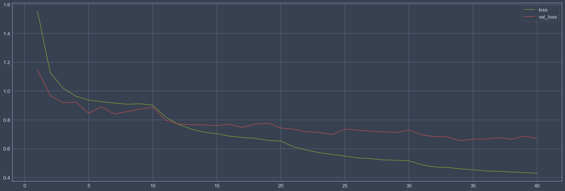
We can see that when changing to a smaller learning rate, the loss drops rapidly (Look at 10, 20, 30 epochs in the loss figure). Which proves that learning rate should match the stage of the model when training.

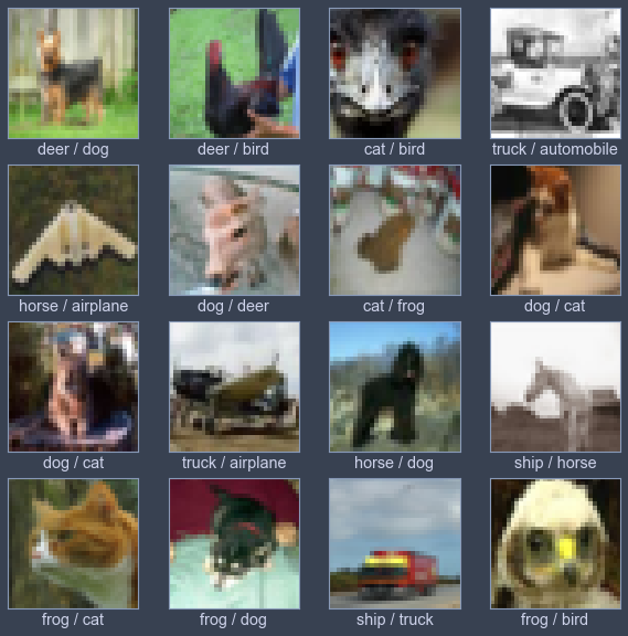
Finally, the most 喜闻乐见 (interesting and funny) part: Error prediction reviewing. I've labeled these data by prediction / correct label